Querying

Hue's goal is to make Databases & Datawarehouses querying easy and productive.

Several apps, each one specialized in a certain type of querying are available. Data sources can be explored first via the browsers.

• The Editor shines for SQL queries. It comes with an intelligent autocomplete, risk alerts and self service troubleshooting.
• The Editor is also available in Notebook mode for quickly executing light programming snippets.
• Dashboards are focusing on visualizing indexed data but can also query SQL databases.

The configuration of the connectors is currently done by the Administrator.

Editor

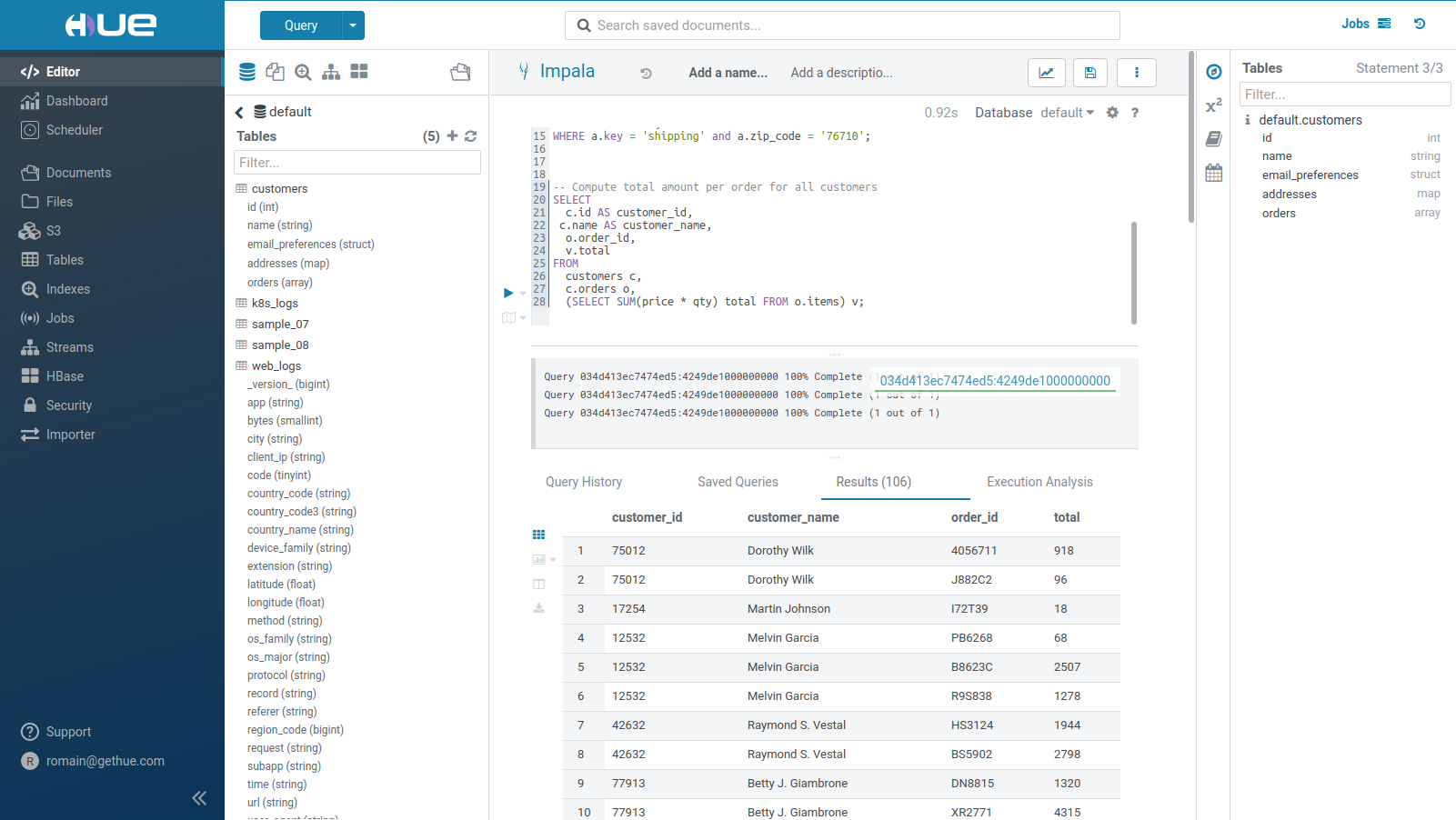
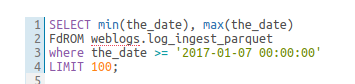
Running Queries

SQL query execution is the primary use case of the Editor. See the list of most common Databases and Datawarehouses.

1. The currently selected statement has a left blue border. To execute a portion of a query, highlight one or more query statements.

2. Click Execute. The Query Results window appears

   • There is a Log caret on the left of the progress bar
   • Expand the Columns by clicking on the column label will scroll to the column. Names and types can be filtered
   • Select the Chart icon to plot the results
   • To expand a row, click on the row number
   • To lock a row, click on the lock icon in the row number column
   • Search either by clicking on the magnifier icon on the results tab, or pressing Ctrl/Cmd + F
   • See more below how to [refine your results](#Refining Results)

3. If there are multiple statements in the query (separated by semi-colons), click Next in the multi-statement query pane to execute the remaining statements.

When you have multiple statements it's enough to put the cursor in the statement you want to execute, the active statement is indicated with a blue gutter marking.

Note: Use CTRL/Cmd + ENTER to execute queries.

Note: On top of the logs panel, there is a link to open the query profile in the Query Browser.

Results

Refining

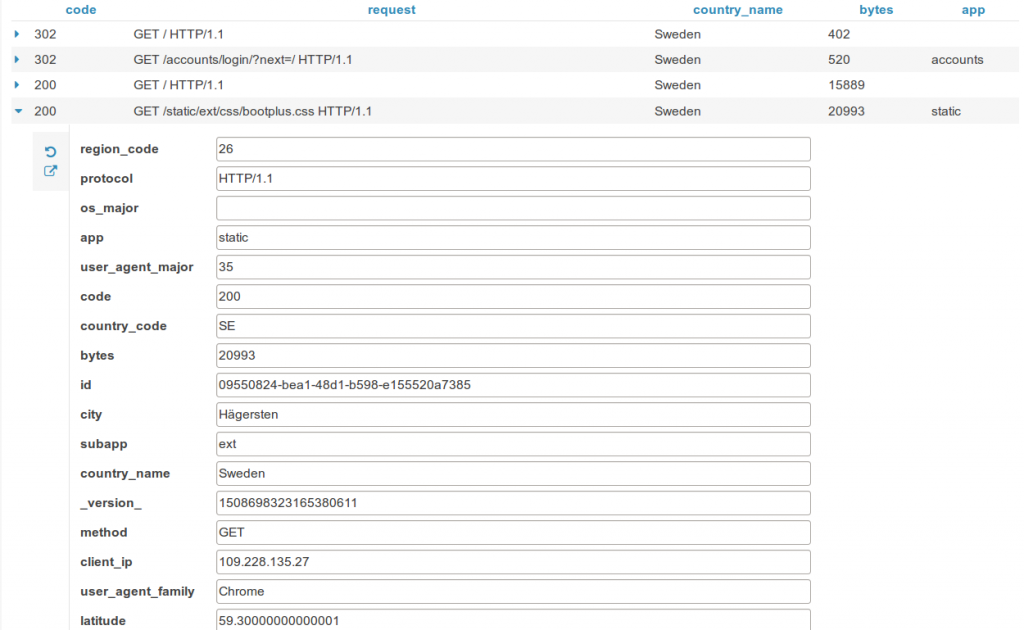
Lock some rows: this will help you compare data with other rows. When you hover a row id, you get a new lock icon. If you click on it, the row automatically sticks to the top of the table.

The column list follows the result grid, can be filtered by data type and can be resized.

The headers of fields with really long content will follow your scroll position and always be visible.

You can now search for certain cell values in the table and the results are highlighted.

You can activate the new search either by clicking on the magnifier icon on the results tab, or pressing Ctrl/Cmd + F.

The virtual renderer display just the cells you need at that moment.

The table you see here has hundreds of columns

If the download to Excel or CSV takes too long, you will have a nice message now

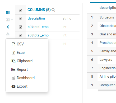
Downloading

There are several ways you can export results of a query.

The most common:

• Download to your computer as a CSV or XLS
• Copy the currently fetched rows to the clipboard

Two of them offer greater scalability:

• Export to an empty folder on your cluster's file system.
• Export to a table. You can choose an already existing table or a new one.

Autocomplete

To make your SQL editing experience, Hue comes with one of the best SQL autocomplete on the planet. The new autocompleter knows all the ins and outs of the Hive and Impala SQL dialects and will suggest keywords, functions, columns, tables, databases, etc. based on the structure of the statement and the position of the cursor.

The result is improved completion throughout. We now have completion for more than just SELECT statements, it will help you with the other DDL and DML statements too, INSERT, CREATE, ALTER, DROP etc.

Smart column suggestions

If multiple tables appear in the FROM clause, including derived and joined tables, it will merge the columns from all the tables and add the proper prefixes where needed. It also knows about your aliases, lateral views and complex types and will include those. It will now automatically backtick any reserved words or exotic column names where needed to prevent any mistakes.

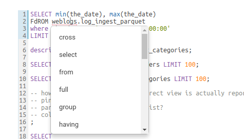
Smart keyword completion

The autocompleter suggests keywords based on where the cursor is positioned in the statement. Where possible it will even suggest more than one word at a time, like in the case of IF NOT EXISTS, no one likes to type too much right? In the parts where order matters but the keywords are optional, for instance after FROM tbl, it will list the keyword suggestions in the order they are expected with the first expected one on top. So after FROM tbl the WHERE keyword is listed above GROUP BY etc.

Functions

The improved autocompleter will now suggest functions, for each function suggestion an additional panel is added in the autocomplete dropdown showing the documentation and the signature of the function. The autocompleter know about the expected types for the arguments and will only suggest the columns or functions that match the argument at the cursor position in the argument list.

Sub-queries, correlated or not

When editing subqueries it will only make suggestions within the scope of the subquery. For correlated subqueries the outside tables are also taken into account.

Context popup

Right click on any fragment of the queries (e.g. a table name) to gets all its metadata information. This is a handy shortcut to get more description or check what types of values are contained in the table or columns.

It’s quite handy to be able to look at column samples while writing a query to see what type of values you can expect. Hue now has the ability to perform some operations on the sample data, you can now view distinct values as well as min and max values. Expect to see more operations in coming releases.

Syntax checker

A little red underline will display the incorrect syntax so that the query can be fixed before submitting. A right click offers suggestions.

Advanced Settings

The live autocompletion is fine-tuned for a better experience advanced settings an be accessed via CTRL + , (or on Mac CMD + ,) or clicking on the ‘?’ icon.

The autocompleter talks to the backend to get data for tables and databases etc and caches it to keep it quick. Clicking on the refresh icon in the left assist will clear the cache. This can be useful if a new table was created outside of Hue and is not yet showing-up (Hue will regularly clear his cache to automatically pick-up metadata changes done outside of Hue).

Sharing

Any query can be shared with permissions, as detailed in the concepts.

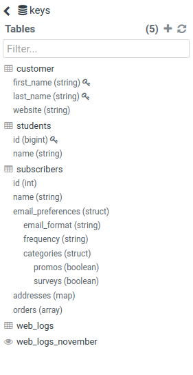
Assist

The Datawarehouse ecosystem is getting more complete with the introduction of transactions. In practice, this means your tables can now support Primary Keys, INSERTs, DELETEs and UPDATEs as well as Partition Keys.

Here is a tutorial demoing how Hue's SQL Editor helps you quickly visualize and use these instructions via its assists and autocomplete components.

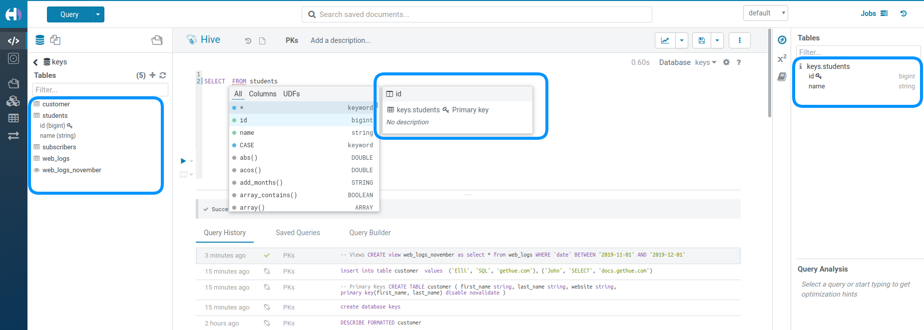
Primary Keys

Primary Keys shows up like Partition Keys with the lock icon:

Here is an example of SQL for using them:

CREATE TABLE customer (
    first_name string,
    last_name string,
    website string,
    PRIMARY KEY (first_name, last_name) DISABLE NOVALIDATE
);

Apache Kudu is supported as well:

CREATE TABLE students (
  id BIGINT,
  name STRING,
  PRIMARY KEY(id)
)
PARTITION BY HASH PARTITIONS 16
STORED AS KUDU
TBLPROPERTIES ('kudu.num_tablet_replicas' = '1')
;

Foreign Keys

When a column value points to another column in another table. e.g. The head of the business unit must exist in the person table:

CREATE TABLE person (
  id INT NOT NULL,
  name STRING NOT NULL,
  age INT,
  creator STRING DEFAULT CURRENT_USER(),
  created_date DATE DEFAULT CURRENT_DATE(),

  PRIMARY KEY (id) DISABLE NOVALIDATE
);

CREATE TABLE business_unit (
  id INT NOT NULL,
  head INT NOT NULL,
  creator STRING DEFAULT CURRENT_USER(),
  created_date DATE DEFAULT CURRENT_DATE(),

  PRIMARY KEY (id) DISABLE NOVALIDATE,
  CONSTRAINT fk FOREIGN KEY (head) REFERENCES person(id) DISABLE NOVALIDATE
);

Partition Keys

Partitioning of the data is a key concept for optimizing the querying. Those special columns are also shown with a key icon:

Here is an example of SQL for using them:

CREATE TABLE web_logs (
    _version_ BIGINT,
    app STRING,
    bytes SMALLINT,
    city STRING,
    client_ip STRING,
    code TINYINT,
    country_code STRING,
    country_code3 STRING,
    country_name STRING,
    device_family STRING,
    extension STRING,
    latitude FLOAT,
    longitude FLOAT,
    `METHOD` STRING,
    os_family STRING,
    os_major STRING,
    protocol STRING,
    record STRING,
    referer STRING,
    region_code BIGINT, request STRING,
    subapp STRING,
    TIME STRING,
    url STRING,
    user_agent STRING,
    user_agent_family STRING,
    user_agent_major STRING,
    id STRING
)
PARTITIONED BY ( `date` STRING);

INSERT INTO web_logs
PARTITION (`date`='2019-11-14') VALUES
(1480895575515725824,'metastore',1041,'Singapore','128.199.234.236',127,'SG','SGP','Singapore','Other',NULL,1.2930999994277954,103.85579681396484,'GET','Other',NULL,'HTTP/1.1',NULL,'-',0,'GET /metastore/table/default/sample_07 HTTP/1.1','table','2014-05-04T06:35:49Z','/metastore/table/default/sample_07','Mozilla/5.0 (compatible; phpservermon/3.0.1; +http://www.phpservermonitor.org)','Other',NULL,'8836e6ce-9a21-449f-a372-9e57641389b3')

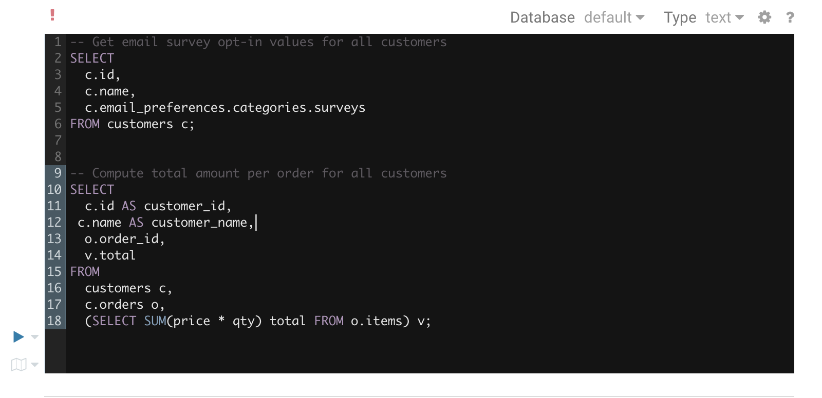
Nested Types

Complex or Nested Types are handy for storing associated data close together. The assist lets you expand the tree of columns:

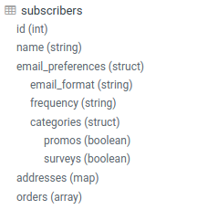
Here is an example of SQL for using them:

CREATE TABLE subscribers (
  id INT,
  name STRING,
  email_preferences STRUCT<email_format:STRING,frequency:STRING,categories:STRUCT<promos:BOOLEAN,surveys:BOOLEAN>>,
  addresses MAP<STRING,STRUCT<street_1:STRING,street_2:STRING,city:STRING,state:STRING,zip_code:STRING>>,
  orders ARRAY<STRUCT<order_id:STRING,order_date:STRING,items:ARRAY<STRUCT<product_id:INT,sku:STRING,name:STRING,price:DOUBLE,qty:INT>>>>
)
STORED AS PARQUET

Views

It can be sometimes confusing to not recognize that a table is instead a view. Views are shown with this little eye icon:

Here is an example of SQL for using them:

CREATE VIEW web_logs_november AS
SELECT * FROM web_logs
WHERE `date` BETWEEN '2019-11-01' AND '2019-12-01'

Transactional Operations

Transactional tables now support these SQL instructions to update the data.

Inserts

Here is how to add some data into a table. Previously, he was only possible to do this via LOADING some files.

INSERT INTO TABLE customer
VALUES
  ('Elli', 'SQL', 'gethue.com'),
  ('John', 'SELECT', 'docs.gethue.com')
;

Deletes

Deletion of rows of data:

DELETE FROM customer
WHERE first_name = 'John';

Updates

How to update the value of some columns in certain rows:

UPDATE customer
SET website = 'helm.gethue.com'
WHERE first_name = 'Elli';

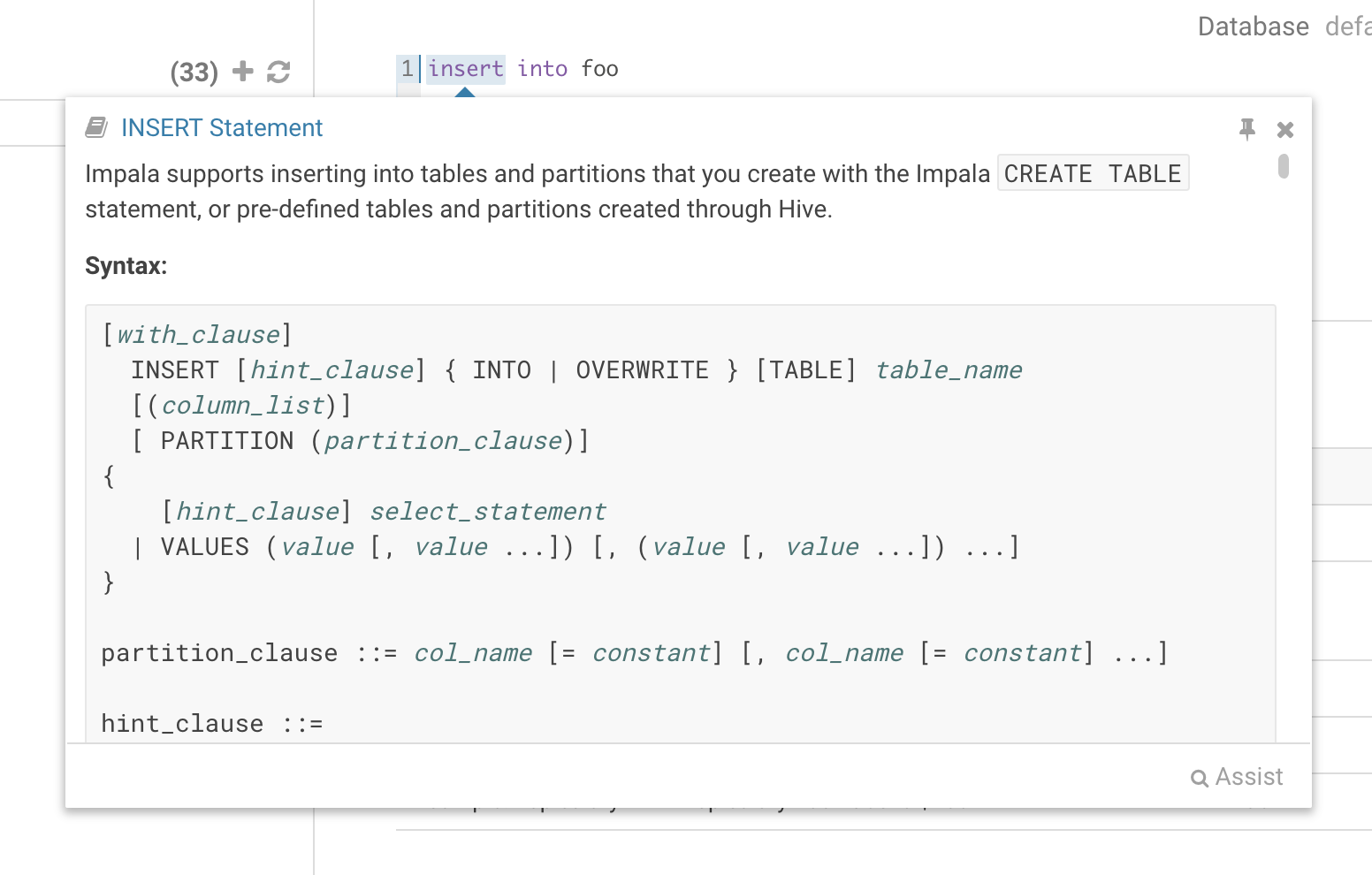
Language reference

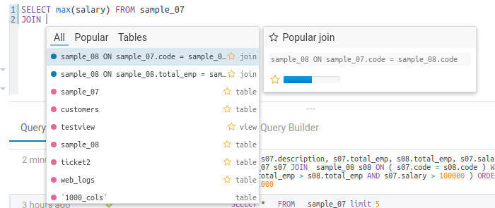
You can find the Language Reference in the right assist panel. The right panel itself has a new look with icons on the left hand side and can be minimised by clicking the active icon.

The filter input on top will only filter on the topic titles in this initial version. Below is an example on how to find documentation about joins in select statements.

While editing a statement there’s a quicker way to find the language reference for the current statement type, just right-click the first word and the reference appears in a popover below:

Variables

Variables are used to easily configure parameters in a query. They are ideal for saving reports that can be shared or executed repetitively:

Single Valued

select * from web_logs where country_code = "${country_code}"

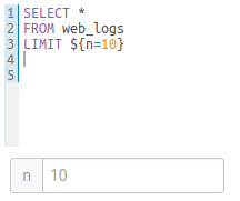
The variable can have a default value

select * from web_logs where country_code = "${country_code=US}"

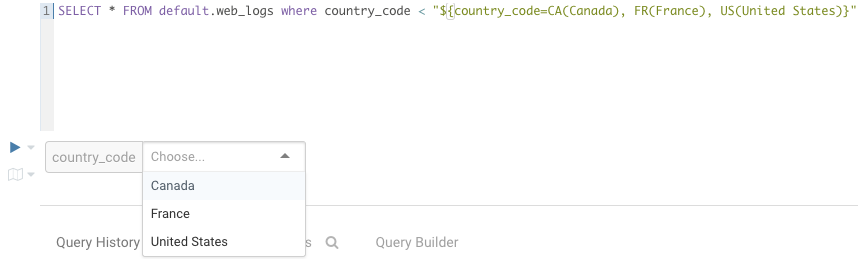
Multi Valued

select * from web_logs where country_code = "${country_code=CA, FR, US}"

In addition, the displayed text for multi valued variables can be changed

select * from web_logs where country_code = "${country_code=CA(Canada), FR(France), US(United States)}"

For values that are not textual, omit the quotes.

select * from boolean_table where boolean_column = ${boolean_column}

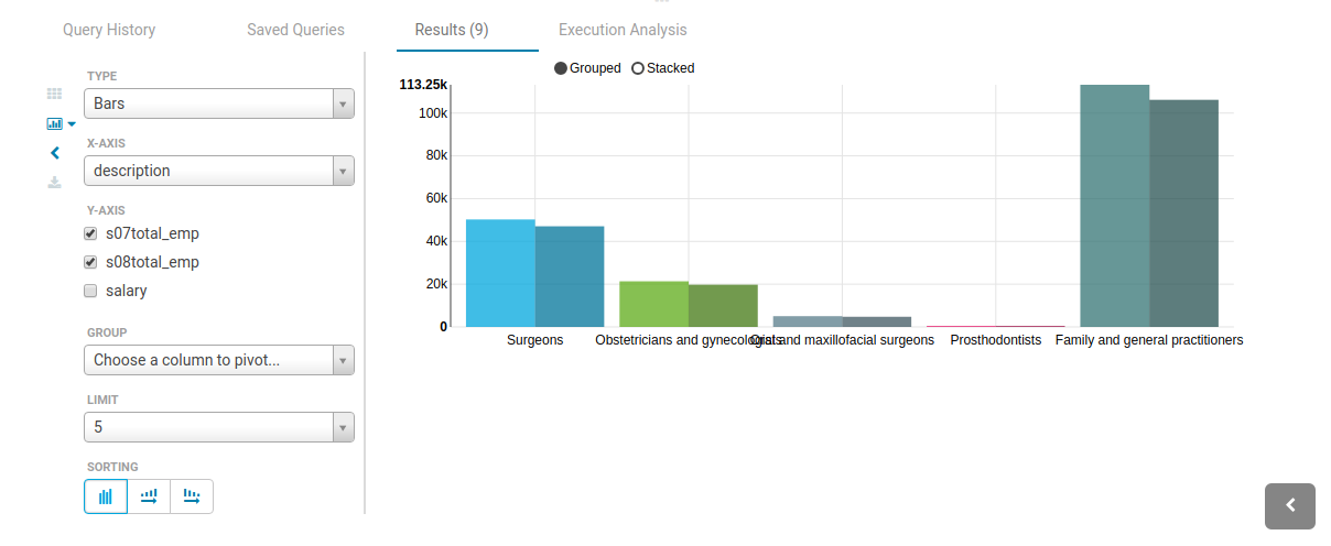
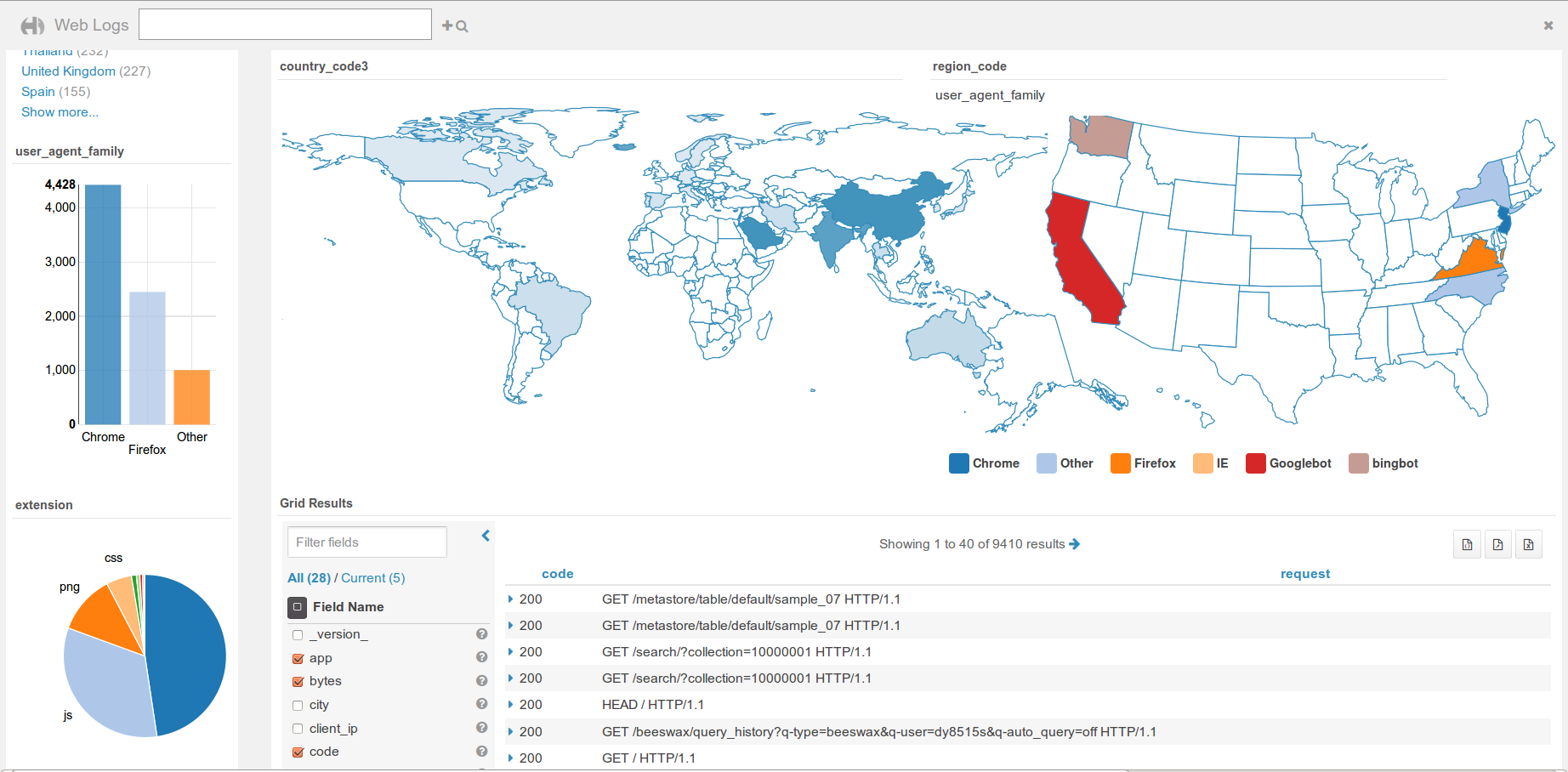
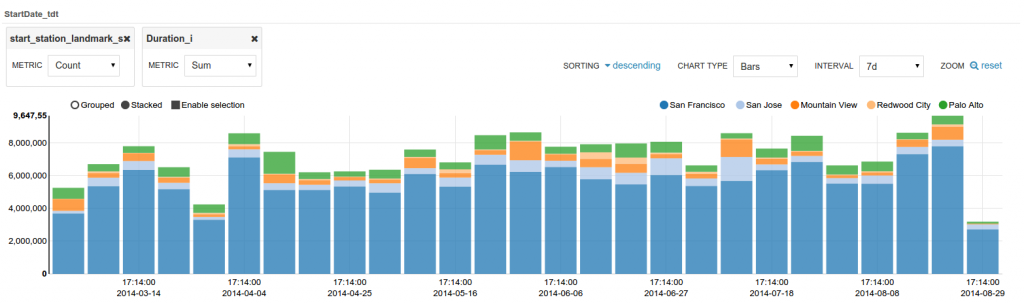
Charting

These visualizations are convenient for plotting chronological data or when subsets of rows have the same attribute: they will be stacked together.

• Pie
• Bar/Line with pivot
• Timeline
• Scattered plot
• Maps (Marker and Gradient)

Query troubleshooting

Pre-query execution

Popular values

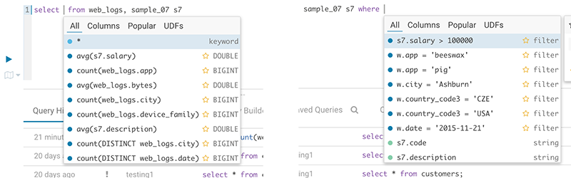
The autocompleter will suggest popular tables, columns, filters, joins, group by, order by etc. based on metadata from Navigator Optimizer. A new “Popular” tab has been added to the autocomplete result dropdown which will be shown when there are popular suggestions available.

This is particularly useful for doing joins on unknown datasets or getting the most interesting columns of tables with hundreds of them.

Risk alerts

While editing, Hue will run your queries through Navigator Optimizer in the background to identify potential risks that could affect the performance of your query. If a risk is identified an exclamation mark is shown above the query editor and suggestions on how to improve it is displayed in the lower part of the right assistant panel.

During execution

The Query Browser details the plan of the query and the bottle necks. When detected, “Health” risks are listed with suggestions on how to fix them.

Tutorial

After finding data in the Catalog and using the Query Assistant, end users might wonder why their queries are taking a lot of time to execute. Build up on top of the Impala profiler, this new feature educates them and surface up more information so that they can be more productive by themselves. Here is a scenario that showcases the flow:

Execution Timeline

To give you a feel for the new features, we’ll execute a few queries.

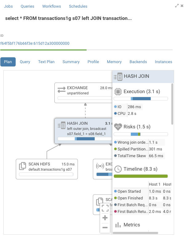
SELECT *
FROM
  transactions1g s07 left JOIN transactions1g s08
ON ( s07.field_1 = s08.field_1) limit 100

transactions1g is a 1GB table and the self join with no predicates will force a network transfer of the whole table.

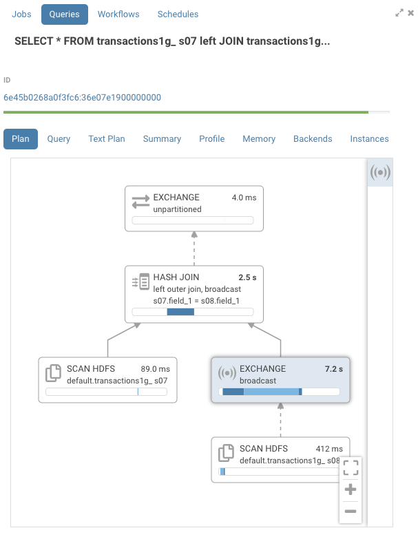
Looking at the profile, you can see a number on the top right of each node that represent its IO and CPU time. There’s also a timeline that gives an estimated representation of when that node was processed during execution. The dark blue color is the CPU time, while the lighter blue is the network or disk IO time. In this example, we can see that the hash join ran for 2.5s. The exchange node, which does the network transfer between 2 hosts, was the most expensive node at 7.2s.

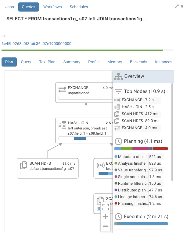
Detail pane

On the right hand side, there is now a pane that is closed by default. To open or close press on the header of the pane. There, you will find a list of all the nodes sorted by execution time, which makes it easier to navigate larger execution graphs. This list is clickable and will navigate to the appropriate node.

Events

Pressing on the exchange node, we find the execution timeline with a bit more detail.

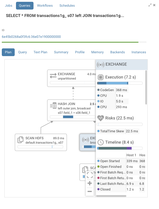
We see that the IO was the most significant portion of the exchange.

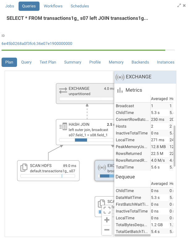
Statistics by host

The detail pane also contains detailed statistics aggregated per host per node such as memory consumption and network transfer speed.

Risks

In the detail pane, for each node, you will find a section titled risks. This section will contain hints on how to improve performance for this operator. Currently, this is not enabled by default. To enable it, go to your Hue ini file and enable this flag:

[notebook]
enable_query_analysis=true

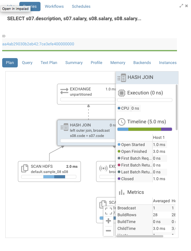
CodeGen

Let’s look at a few queries and some of the risks that can be identified.

SELECT s07.description, s07.salary, s08.salary,
  s08.salary - s07.salary
FROM
  sample_07 s07 left outer JOIN sample_08 s08
ON ( s07.code = s08.code)
where s07.salary > 100000

sample_07 & sample_08 are small sample tables that come with Hue.

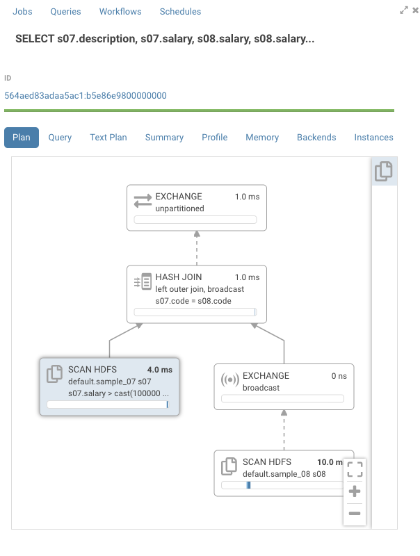
Looking at the graph, the timelines are mostly empty. If we open one of the nodes we see that all the time is taken by “CodeGen”.

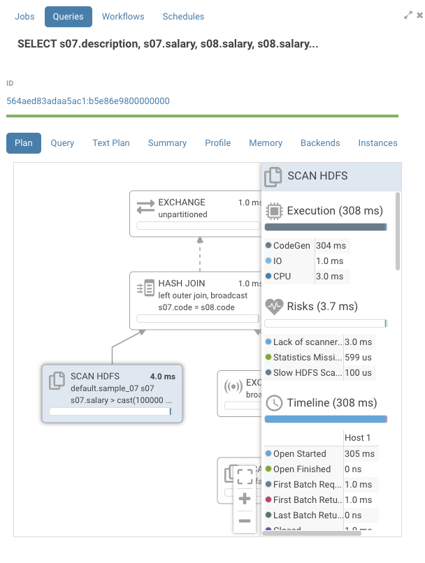
Impala compiles SQL requests to native code to execute each node in the graph. On queries with large table this gives a large performance boost. On smaller tables, we can see that CodeGen is the main contributor to execution time. Normally, Impala disables CodeGen with tables of small sizes, but Impala doesn’t know it’s a small table as is pointed out in the risks section by the statement “Statistics missing”. Two solutions are available here:

Adding the missing statistics. One way to do this is to execute the following command:

compute stats sample_07;
compute stats sample_08;

This is usually the right thing to do, but on larger tables it can be quite expensive.

Disable codegen for the query via:

set DISABLE_CODEGEN=true

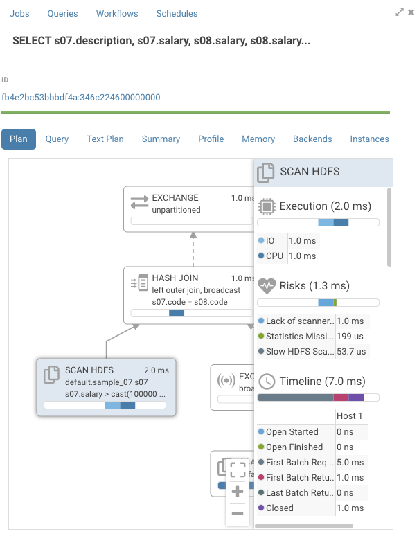
After rerunning the query, we see that CodeGen is now gone.

Join Order

If we open the join node, there’s a warning for wrong join order.

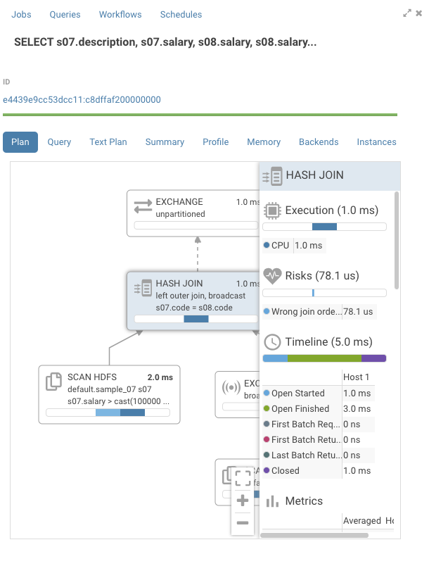
Impala prefers having the table with the larger size on the right hand side of the graph, but in this case the reverse is true. Normally, Impala would optimize this automatically, but we saw that the statistics were missing for the tables being joined. There a few ways we could fix this:

• Add the missing statistics as described earlier.

• Rewrite the query the change the join order:

  SELECT s07.description, s07.salary, s08.salary,
    s08.salary - s07.salary
  FROM
    sample_08 s08 left outer JOIN sample_07 s07
  ON ( s07.code = s08.code)
  where s07.salary > 100000
  

The warning is gone and the execution time for the join is down.

Spilling

Impala will execute all of its operators in memory if enough is available. If the execution does not all fit in memory, Impala will use the available disk to store its data temporarily. To see this in action, we’ll use the same query as before, but we’ll set a memory limit to trigger spilling:

set MEM_LIMIT=1g;
select *
FROM
  transactions1g s07 left JOIN transactions1g s08
ON ( s07.field_1 = s08.field_1);

Looking at the join node, we can see that there’s an entry in the risk section about a spilled partition. Typically, the join only has CPU time, but in this case it also has IO time due to the spill.

Kudu Filtering

Kudu is one of the supported storage backends for Impala. While Impala stand alone can query a variety of file data formats, Impala on Kudu allows fast updates and inserts on your data, and also is a better choice if small files are involved. When using Impala on Kudu, Impala will push down some of the operations to Kudu to reduce the data transfer between the two.

However, Kudu does not support all the operators that Impala support. For example, at the time of writing, Impala support the ‘like’ operator, but Kudu does not. In those cases, all the data that cannot be natively filtered in Kudu is transferred to Impala where it will be filtered. Let’s look at a behavior difference between the two.

SELECT * FROM transactions1g_kudu s07 left JOIN transactions1g_kudu s08 on s07.field_1 = s08.field_1
where s07.field_5 LIKE '2000-01%';

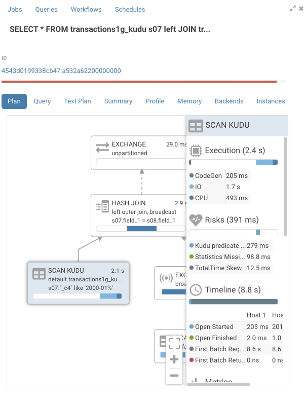
When we look at the graph, we see that on the Kudu node we have both IO, which represent the time spent in Kudu, and CPU, which represent the time spent in Impala, for a total of 2.1s. In the risk section, we can also find a warning that Kudu could not evaluate the predicate.

SELECT * FROM transactions1g_kudu s07 left JOIN transactions1g_kudu s08 on s07.field_1 = s08.field_1
where s07.field_5 <= '2000-01-31' and s07.field_5 >= '2000-01-01';

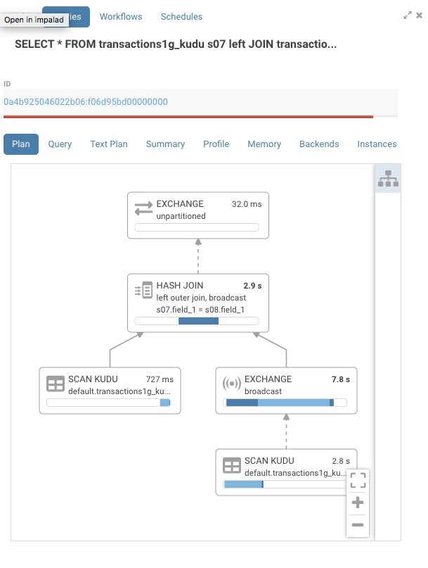
When we look a the graph, we see that on the Kudu node now mostly has IO for a total time 727ms.

Others

You might also have queries where the nodes have short execution time, but the total duration time is long. Using the same query, we see all the nodes have sub 10ms execution time, but the query execution was 7.9s.

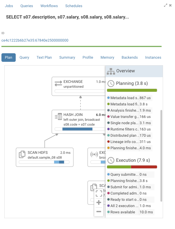
Looking at the global timeline, we see that the planning phase took 3.8s with most of the time in metadata load. When Impala doesn’t have metadata about a table, which can happen after a user executes:

invalidate metadata;

Impala has to refetch the metadata from the metastore. Furthermore, we see that the second most expensive item at 4.1s is first row fetched. This is the time it took the client, Hue in this case, to fetch the results. While both of these events are not things that a user can change, it’s good to see where the time is spent.

Post-query execution

A new experimental panel when enabled can offer post risk analysis and recommendation on how to tweak the query for better speed.

Modes

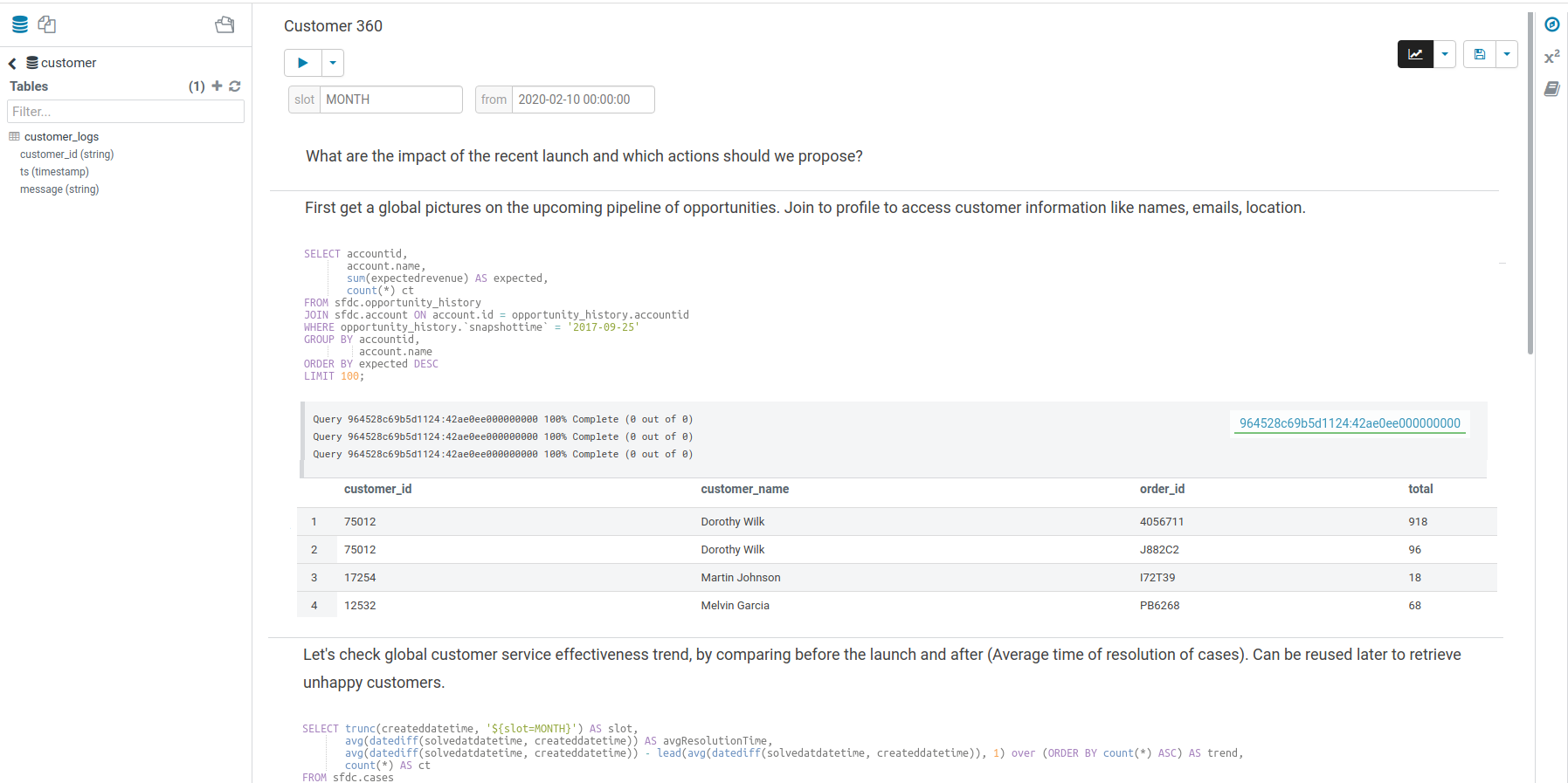
Presentation

Turns a list of semi-colon separated queries into an interactive presentation by clicking on the ‘Dashboard’ icon. It is great for doing presentations with a scenario and live results to prove a point or executing reports containting a suite of sequential queries in one click.

Dark

Initially this mode is limited to the actual editor area and we’re considering extending this to cover all of Hue.

To toggle the dark mode you can either press Ctrl-Alt-T or Command-Option-T on Mac while the editor has focus. Alternatively you can control this through the settings menu which is shown by pressing Ctrl-, or Command-, on Mac.

Dashboard

Dashboards provide an interactive way to query indexed data quickly and easily. No programming is required and the analysis is done by drag & drops and clicks.

Widgets are interconnected together. This is great for exploring new datasets or monitoring without having to type.

The best supported engine is Apache Solr, then support for SQL databases is getting better. To help add more SQL support, feel free to check the dashboard connector section.

These tutorials showcase the capabilities:

• The top search bar offers a full autocomplete on all the values of the index
• Seeing real time data
• Comprehensive demo of BikeShare data visualization post

Analytics facets

Drill down the dimensions of the datasets and apply aggregates functions on top of it:

Some facets can be nested:

Autocomplete

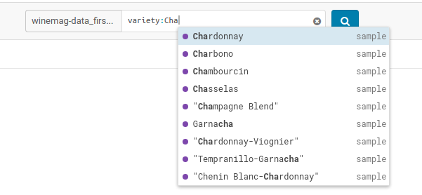
The top bar support faceted and free word text search, with autocompletion.

Marker Map

Points close to each other are grouped together and will expand when zooming-in. A Yelp-like search filtering experience can also be created by checking the box.

Edit records

Indexed records can be directly edited in the Grid or HTML widgets by admins.

Links

Links to the original documents can also be inserted. Add to the record a field named ‘link-meta’ that contains some json describing the URL or address of a table or file that can be open in the HBase Browser, Metastore App or File Browser:

Any link

{'type': 'link', 'link': 'gethue.com'}

HBase Browser

{'type': 'hbase', 'table': 'document_demo', 'row_key': '20150527'}
{'type': 'hbase', 'table': 'document_demo', 'row_key': '20150527', 'fam': 'f1'}
{'type': 'hbase', 'table': 'document_demo', 'row_key': '20150527', 'fam': 'f1', 'col': 'c1'}

File Browser

{'type': 'hdfs', 'path': '/data/hue/file.txt'}

Table Catalog

{'type': 'hive', 'database': 'default', 'table': 'sample_07'}

Saved queries

Current selected facets and filters, query strings can be saved with a name within the dashboard. These are useful for defining “cohorts” or pre-selection of records and quickly reloading them.

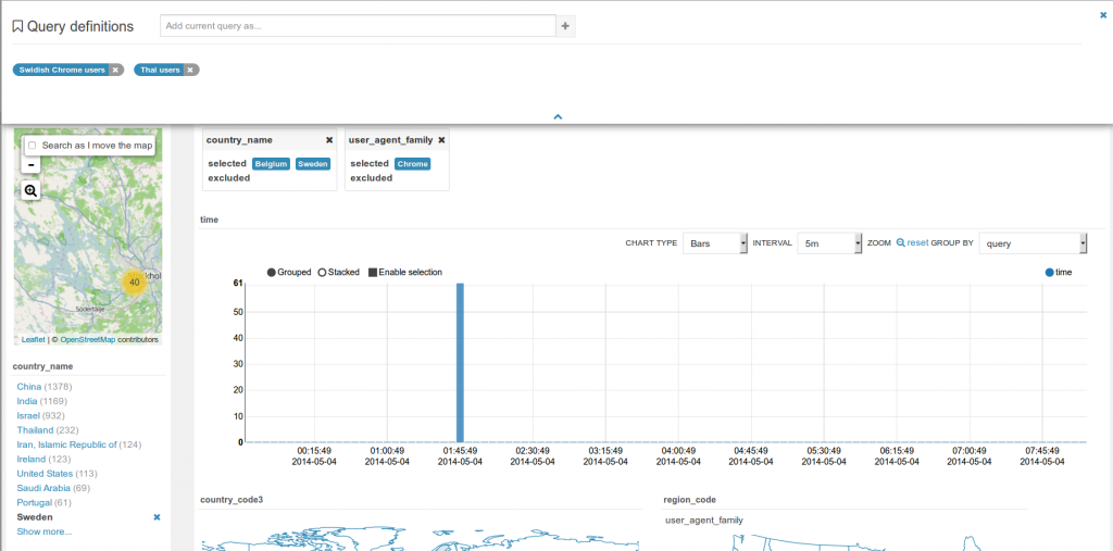
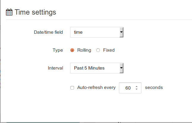
‘Fixed’ or ‘rolling’ window

Real time indexing can now shine with the rolling window filter and the automatic refresh of the dashboard every N seconds. See it in action in the real time Twitter indexing with Spark streaming post.

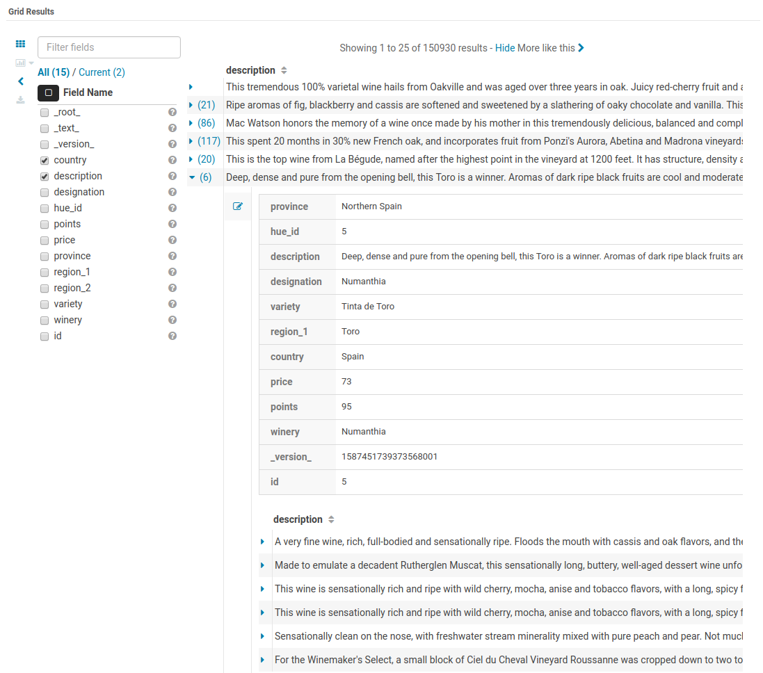
‘More like this’

This feature lets you selected fields you would like to use to find similar records. This is a great way to find similar issues, customers, people… with regard to a list of attributes.

Notebook

The goal of Notebooks is to quickly experiment with small programming snippets (with in particular Spark) and do interactive demos. Its goal is to stay lightweight with regards to other notebook or programming systems.

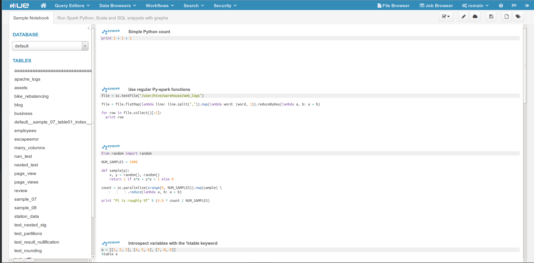
The main advantage is to be able to add snippets of different dialects (e.g. PySpark, Hive SQL…) into a single page:

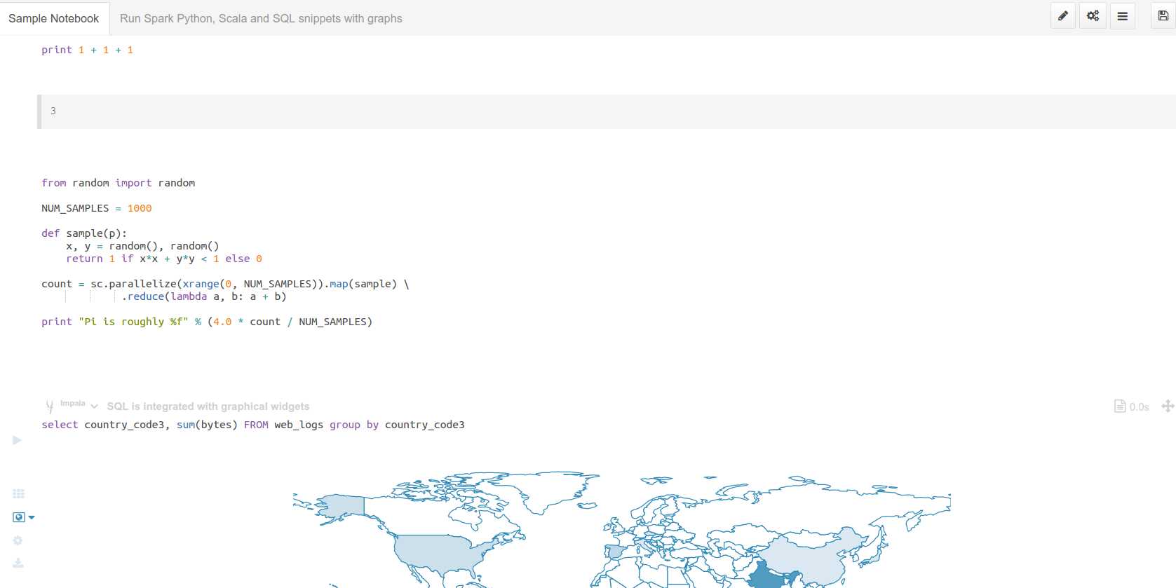
Any configured language of the Editor will be available as a dialect. Each snippet has a code editor, with autocomplete, syntax highlighting and other feature like shortcut links to HDFS paths and Hive tables.

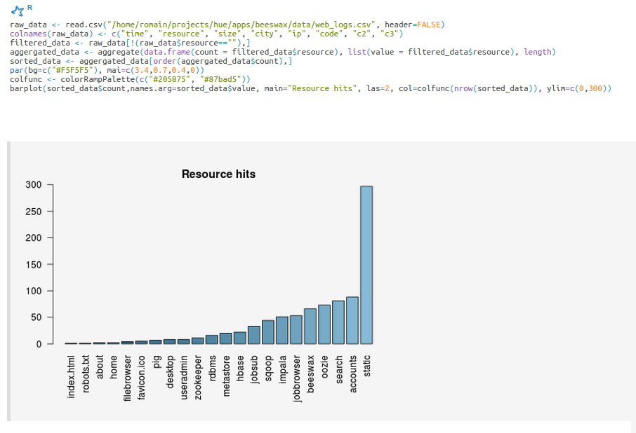
Example of SparkR shell with inline plot

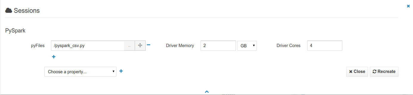
All the spark-submit, spark-shell, pyspark, sparkR properties of jobs & shells can be added to the sessions of a Notebook. This will for example let you add files, modules and tweak the memory and number of executors.

Spark

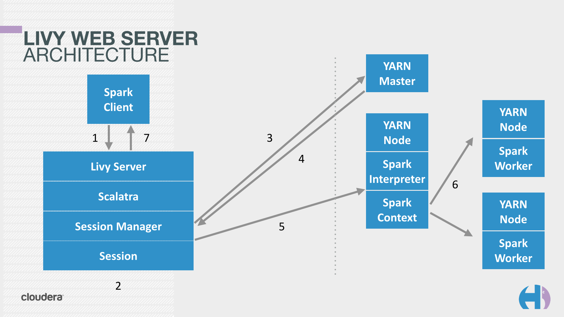
Hue relies on Livy for the interactive Scala, Python, SparkSQL and R snippets.

Livy is an open source REST interface for interacting with Apache Spark from anywhere. It got initially developed in the Hue project but got a lot of traction and was moved to its own project on livy.io.

Make sure that the Notebook and interpreters configured.

Livy

Starting the Livy REST server is detailed on the get started page.

Executing some Spark

As the REST server is running, we can communicate with it. We are on the same machine so will use ‘localhost’ as the address of Livy.

Let’s list our open sessions

curl localhost:8998/sessions

{"from":0,"total":0,"sessions":[]}

Note You can use

| python -m json.tool

at the end of the command to prettify the output, e.g.:

curl localhost:8998/sessions/0 | python -m json.tool

There is zero session. We create an interactive PySpark session

curl -X POST --data '{"kind": "pyspark"}' -H "Content-Type: application/json" localhost:8998/sessions

{"id":0,"state":"starting","kind":"pyspark","log":[]}

Sessions ids are incrementing numbers starting from 0. We can then reference the session later by its id.

We check the status of the session until its state becomes idle: it means it is ready to be execute snippet of PySpark:

curl localhost:8998/sessions/0 | python -m json.tool


% Total    % Received % Xferd  Average Speed   Time    Time     Time  Current

                                Dload  Upload   Total   Spent    Left  Speed

100  1185    0  1185    0     0  72712      0 --:--:-- --:--:-- --:--:-- 79000

{

    "id": 5,

    "kind": "pyspark",

    "log": [

      "15/09/03 17:44:14 INFO util.Utils: Successfully started service 'SparkUI' on port 4040.",

      "15/09/03 17:44:14 INFO ui.SparkUI: Started SparkUI at http://172.21.2.198:4040",

      "15/09/03 17:44:14 INFO spark.SparkContext: Added JAR file:/home/romain/projects/hue/apps/spark/java-lib/livy-assembly.jar at http://172.21.2.198:33590/jars/livy-assembly.jar with timestamp 1441327454666",

      "15/09/03 17:44:14 WARN metrics.MetricsSystem: Using default name DAGScheduler for source because spark.app.id is not set.",

      "15/09/03 17:44:14 INFO executor.Executor: Starting executor ID driver on host localhost",

      "15/09/03 17:44:14 INFO util.Utils: Successfully started service 'org.apache.spark.network.netty.NettyBlockTransferService' on port 54584.",

      "15/09/03 17:44:14 INFO netty.NettyBlockTransferService: Server created on 54584",

      "15/09/03 17:44:14 INFO storage.BlockManagerMaster: Trying to register BlockManager",

      "15/09/03 17:44:14 INFO storage.BlockManagerMasterEndpoint: Registering block manager localhost:54584 with 530.3 MB RAM, BlockManagerId(driver, localhost, 54584)",

      "15/09/03 17:44:15 INFO storage.BlockManagerMaster: Registered BlockManager"

    ],

    "state": "idle"

}

Session properties

All the properties supported by spark shells like the number of executors, the memory, etc can be changed at session creation. Their format is the same as when typing spark-shell -h

curl -X POST --data '{"kind": "pyspark", "numExecutors": "3", "executorMemory": "2G"}' -H "Content-Type: application/json" localhost:8998/sessions
{"id":0,"state":"starting","kind":"pyspark","numExecutors":"3","executorMemory":"2G","log":[]}

Executing statements

In YARN mode, Livy creates a remote Spark Shell in the cluster that can be accessed easily with REST

When the session state is idle, it means it is ready to accept statements! Lets compute 1 + 1

curl localhost:8998/sessions/0/statements -X POST -H 'Content-Type: application/json' -d '{"code":"1 + 1"}'

{"id":0,"state":"running","output":null}

We check the result of statement 0 when its state is available

curl localhost:8998/sessions/0/statements/0

{"id":0,"state":"available","output":{"status":"ok","execution_count":0,"data":{"text/plain":"2"}}}

Note If the statement is taking less than a few milliseconds, Livy returns the response directly in the response of the POST command.

Statements are incrementing and all share the same context, so we can have a sequences

curl localhost:8998/sessions/0/statements -X POST -H 'Content-Type: application/json' -d '{"code":"a = 10"}'

{"id":1,"state":"available","output":{"status":"ok","execution_count":1,"data":{"text/plain":""}}}

Spanning multiple statements

curl localhost:8998/sessions/5/statements -X POST -H 'Content-Type: application/json' -d '{"code":"a + 1"}'

{"id":2,"state":"available","output":{"status":"ok","execution_count":2,"data":{"text/plain":"11"}}}

Let’s close the session to free up the cluster. Note that Livy will automatically inactive idle sessions after 1 hour (configurable).

curl localhost:8998/sessions/0 -X DELETE

{"msg":"deleted"}

Tutorial: Sharing RDDs

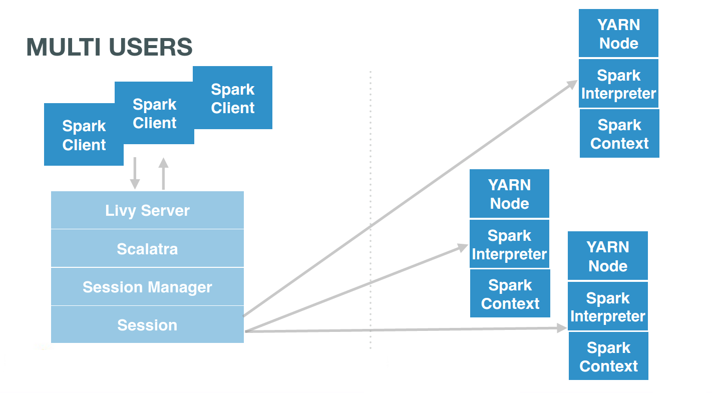
This section shows how to share Spark RDDs and contexts. Livy offers remote Spark sessions to users. They usually have one each (or one by Notebook):

# Client 1
curl localhost:8998/sessions/0/statements -X POST -H 'Content-Type: application/json' -d '{"code":"1 + 1"}'
# Client 2
curl localhost:8998/sessions/1/statements -X POST -H 'Content-Type: application/json' -d '{"code":"..."}'
# Client 3
curl localhost:8998/sessions/2/statements -X POST -H 'Content-Type: application/json' -d '{"code":"..."}'
livy_shared_contexts2

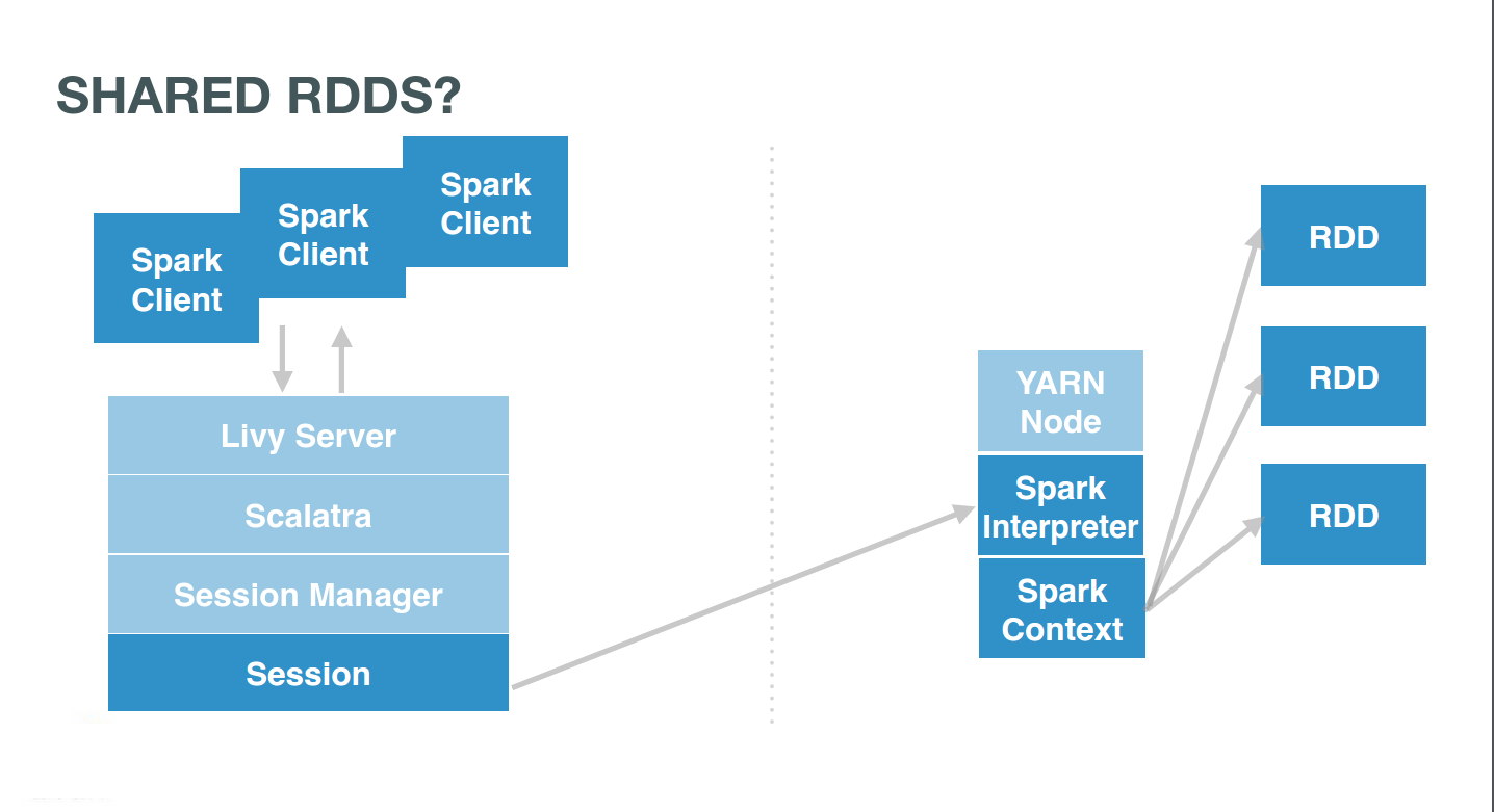
… and so sharing RDDs

If the users were pointing to the same session, they would interact with the same Spark context. This context would itself manages several RDDs. Users simply need to use the same session id, e.g. 0, and issue commands there:

# Client 1
curl localhost:8998/sessions/0/statements -X POST -H 'Content-Type: application/json' -d '{"code":"1 + 1"}'

# Client 2
curl localhost:8998/sessions/0/statements -X POST -H 'Content-Type: application/json' -d '{"code":"..."}'

# Client 3
curl localhost:8998/sessions/0/statements -X POST -H 'Content-Type: application/json' -d '{"code":"..."}'

…Accessing them from anywhere

Now we can even make it more sophisticated while keeping it simple. Imagine we want to simulate a shared in memory key/value store. One user can start a named RDD on a remote Livy PySpark session and anybody could access it.

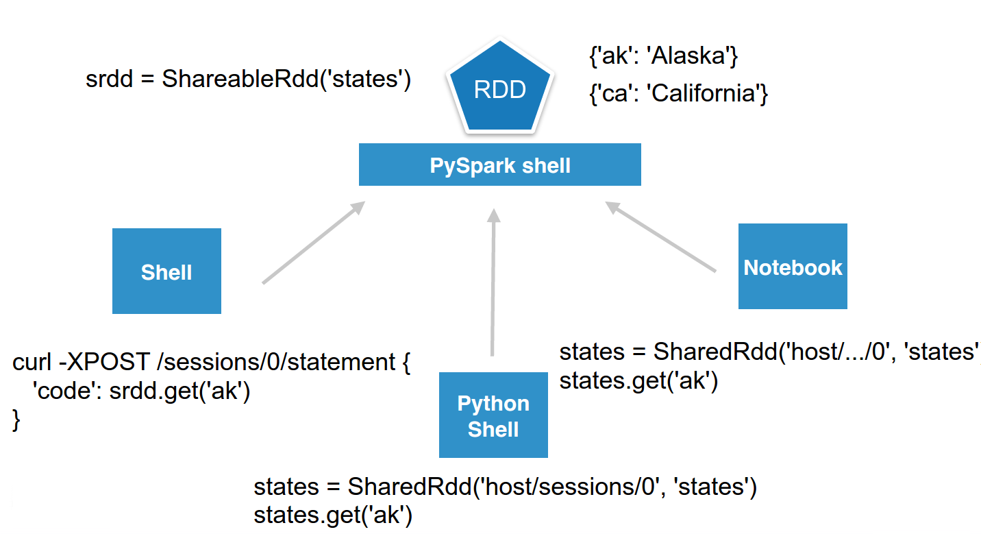
To make it prettier, we can wrap it in a few lines of Python and call it ShareableRdd. Then users can directly connect to the session and set or retrieve values.

class ShareableRdd():

def __init__(self):
  self.data = sc.parallelize([])

def get(self, key):
  return self.data.filter(lambda row: row[0] == key).take(1)

def set(self, key, value):
  new_key = sc.parallelize([[key, value]])
  self.data = self.data.union(new_key)

set() adds a value to the shared RDD, while get() retrieves it.

srdd = ShareableRdd()

srdd.set('ak', 'Alaska')
srdd.set('ca', 'California')

srdd.get('ak')

If using the REST Api directly someone can access it with just these commands:

curl localhost:8998/sessions/0/statements -X POST -H 'Content-Type: application/json' -d '{"code":"srdd.get(\"ak\")"}'
{"id":3,"state":"running","output":null}

curl localhost:8998/sessions/0/statements/3
{"id":3,"state":"available","output":{"status":"ok","execution_count":3,"data":{"text/plain":"[['ak', 'Alaska']]"}}}

We can even get prettier data back, directly in json format by adding the %json magic keyword:

curl localhost:8998/sessions/0/statements -X POST -H 'Content-Type: application/json' -d  '{"code":"data = srdd.get(\"ak\")\n%json data"}'
{"id":4,"state":"running","output":null}

curl localhost:8998/sessions/0/statements/4
{"id":4,"state":"available","output":{"status":"ok","execution_count":2,"data":{"application/json":[["ak","Alaska"]]}}}

Even from any languages

As Livy is providing a simple REST Api, we can quickly implement a little wrapper around it to offer the shared RDD functionality in any languages. Let’s do it with regular Python:

pip install requests
python

Then in the Python shell just declare the wrapper:

import requests
import json

class SharedRdd():
  """
  Perform REST calls to a remote PySpark shell containing a Shared named RDD.
  """
  def __init__(self, session_url, name):
    self.session_url = session_url
    self.name = name

  def get(self, key):
    return self._curl('%(rdd)s.get("%(key)s")' % {'rdd': self.name, 'key': key})

  def set(self, key, value):
    return self._curl('%(rdd)s.set("%(key)s", "%(value)s")' % {'rdd': self.name, 'key': key, 'value': value})

  def _curl(self, code):
    statements_url = self.session_url + '/statements'
    data = {'code': code}
    r = requests.post(statements_url, data=json.dumps(data), headers={'Content-Type': 'application/json'})
    resp = r.json()
    statement_id = str(resp['id'])
    while resp['state'] == 'running':
      r = requests.get(statements_url + '/' + statement_id)
      resp = r.json()
    return r.json()['data']

Instantiate it and make it point to a live session that contains a ShareableRdd:

states = SharedRdd('http://localhost:8998/sessions/0', 'states')

And just interact with the RDD transparently:

states.get('ak')
states.set('hi', 'Hawaii')

Others

Apache Pig Type Apache Pig latin instructions to load/merge data to perform ETL or Analytics.

Apache Sqoop Run an SQL import from a traditional relational database via an Apache Sqoop command.